Carbon dioxide removal & solar radiation modification


This post takes a quick look at carbon dioxide removal (CDR) and solar radiation modification (SRM). For detailed explanations, links to the source articles (such as IPCC report chapters) are at the bottom.


Carbon dioxide removal (CDR)


Carbon dioxide removal (CDR) is defined as “Anthropogenic activities removing carbon dioxide (CO2) from the atmosphere and durably storing it in geological, terrestrial, or ocean reservoirs, or in products. It includes existing and potential anthropogenic enhancement of biological or geochemical CO2 sinks and direct air carbon dioxide capture and storage (DACCS), but excludes natural CO2 uptake not directly caused by human activities.”

Source: IPCC (2021) AR6 WGI Annex VII, Glossary, pg. 2221


“Within ambitious mitigation strategies at global or national levels, CDR cannot serve as a substitute for deep emissions reductions but can fulfil multiple complementary roles: it can (i) further reduce net CO2 or GHG emission levels in the near-term; (ii) counterbalance residual emissions from hard-to-transition sectors, such as CO2 from industrial activities and long-distance transport (e.g., aviation, shipping), or methane and nitrous oxide from agriculture, in order to help reach net zero CO2 or GHG emissions in the mid-term; (iii) achieve and sustain net-negative CO2 or GHG emissions in the long-term, by deploying CDR at levels exceeding annual residual gross CO2 or GHG emissions”

Source: IPCC (2022) AR6 WGIII Chapter 12, Cross-Chapter Box 8, pg. 1262


“All available studies require at least some kind of carbon dioxide removal to reach net zero; that is, there are no studies where absolute zero GHG or even CO2 emissions are reached by deep emissions reductions alone.”

Source: IPCC (2022) AR6 WGIII Chapter 3, FAQ 3.2, pg. 385


Carbon dioxide removal taxonomy
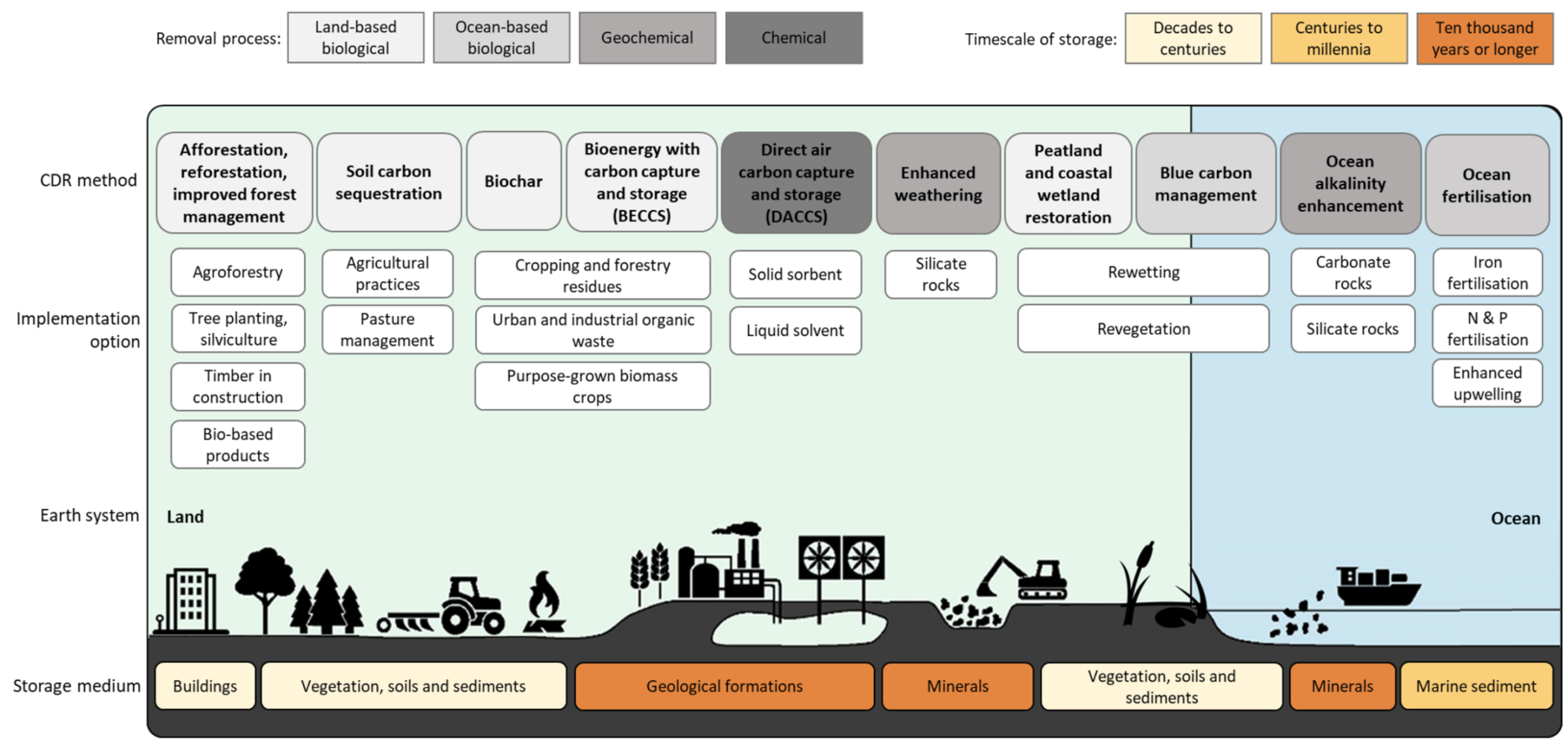
A detailed taxonomy diagram illustrating various Carbon Dioxide Removal methods, categorised by removal process, implementation options, Earth system, and storage medium. The graphic is divided horizontally into Land and Ocean systems. For the Land system, biological removal processes include Afforestation, reforestation, and improved forest management; Soil carbon sequestration; Biochar; Bioenergy with carbon capture and storage; and Peatland and coastal wetland restoration. Chemical and geochemical land methods include Direct air carbon capture and storage, and Enhanced weathering. In the Ocean system, methods include Blue carbon management, Ocean alkalinity enhancement, and Ocean fertilisation. Below each method, specific implementation options are listed, ranging from agroforestry and solid sorbents to N and P fertilisation. A landscape illustration at the bottom displays icons like trees, tractors, factories, and ships to visually represent the methods in action. Below this, a colour-coded band categorises the resulting storage mediums by their timescale. Buildings, vegetation, soils, and sediments provide storage for decades to centuries. Marine sediments offer storage for centuries to millennia. Finally, geological formations and minerals provide the longest storage timescales, lasting ten thousand years or longer.
Cross-Chapter Box 8, Figure 1:  Methods are categorised based on removal process (grey shades) and storage medium (for which timescales of storage are given, yellow/brown shades). Main implementation options are included for each CDR method. Note that specific land-based implementation options can be associated with several CDR methods, for example, agroforestry can support soil carbon sequestration and provide biomass for biochar or BECCS. Source: adapted from Minx et al. (2018).
Source: IPCC (2022) AR6 WGIII Chapter 12, Cross-Chapter Box 8, Figure 1, pg. 1262

“Most modelled pathways that likely limit warming to 2°C (>67%) above pre-industrial levels and below use land-based CO2 removal such as afforestation/reforestation and BECCS to achieve net zero CO2 and net zero GHG emissions even while some CO2 and non-CO2 emissions continue to occur. Pathways with more demand-side interventions that limit the amount of energy we use, or where the diet that we consume is changed, can achieve net zero CO2, or net zero GHG emissions with less carbon dioxide removal (CDR).”

Source: IPCC (2022) AR6 WGIII Chapter 3, FAQ 3.2, pg. 385


“Deliberate carbon dioxide removal (CDR) from the atmosphere has the potential to compensate for residual CO2 emissions to reach net zero CO2 emissions or to generate net negative CO2 emissions. In the same way that part of current anthropogenic net CO2 emissions are taken up by land and ocean carbon stores, net CO2 removal will be partially counteracted by CO2 release from these stores (very high confidence). Asymmetry in the carbon cycle response to simultaneous CO2 emissions and removals implies that a larger amount of CO2 would need to be removed to compensate for an emission of a given magnitude to attain the same change in atmospheric CO2 (medium confidence). CDR methods have wide-ranging side-effects that can either weaken or strengthen the carbon sequestration and cooling potential of these methods and affect the achievement of sustainable development goals (high confidence).”

Source: IPCC (2021) AR6 WGI TS.3.3.2, pg. 99


“Approaches capable of large-scale removal of CO2 are still in the state of research and development or unproven at the scales of deployment necessary to achieve a net reduction in atmospheric CO2 levels. CO2 removal approaches, particularly those deployed on land, can have undesired side effects on water, food production and biodiversity.”

Source: IPCC (2021) AR6 WGI Chapter 5, FAQ 5.3, pg. 776


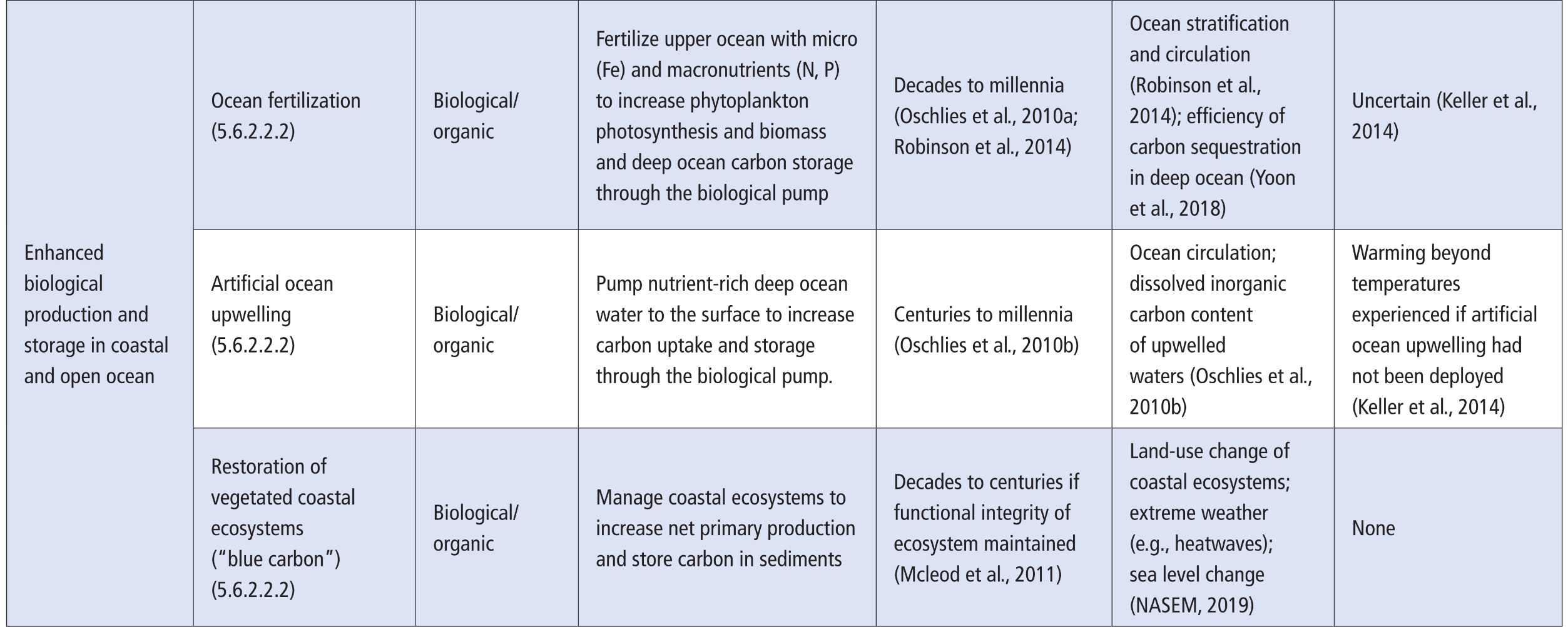
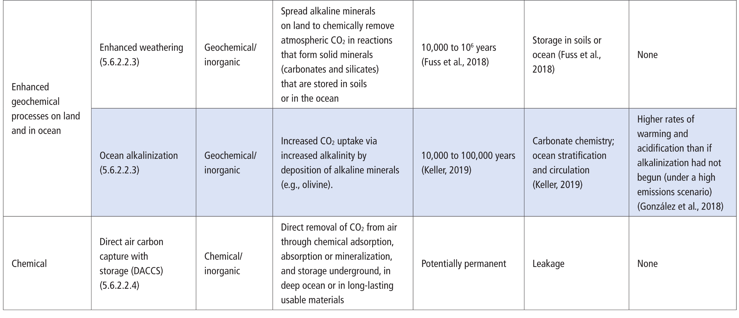
Characteristics of carbon dioxide removal (CDR) methods
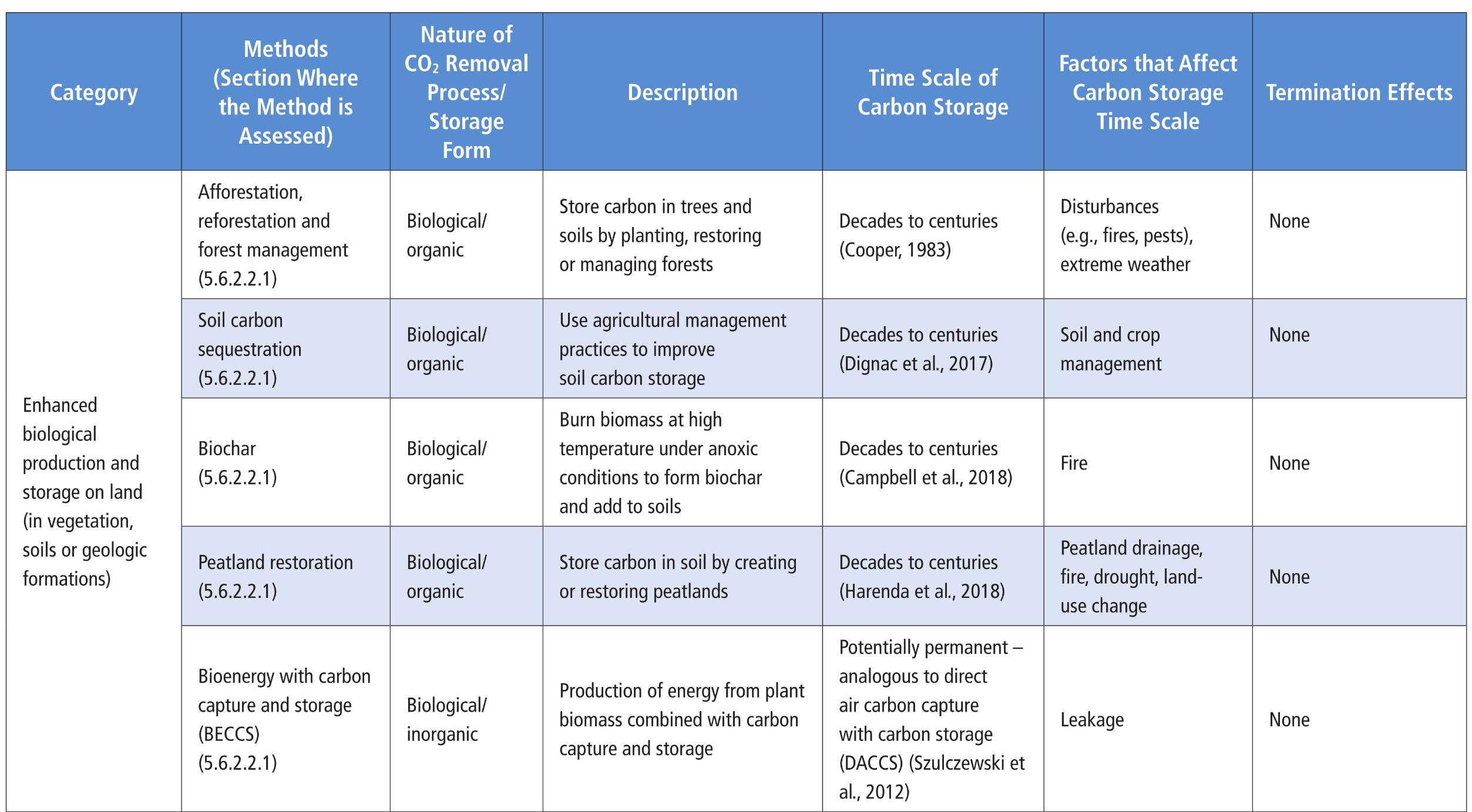
A comprehensive data table categorising eleven carbon dioxide removal methods based on their characteristics. The table is divided into columns tracking the Method, Nature of the removal process and storage form, Description, Time Scale of Carbon Storage, Factors that Affect the Time Scale, and Termination Effects. The methods are grouped into four overarching categories. First, enhanced biological production and storage on land includes afforestation, soil carbon sequestration, biochar, peatland restoration, and bioenergy with carbon capture and storage. Their storage timescales generally range from decades to centuries, except for bioenergy which is potentially permanent, and none show termination effects. Second, enhanced biological production and storage in coastal and open ocean includes ocean fertilisation, artificial ocean upwelling, and restoration of vegetated coastal ecosystems. These offer storage from decades up to millennia, but ocean fertilisation and artificial upwelling carry uncertain or warming termination effects. Third, enhanced geochemical processes on land and in the ocean include enhanced weathering and ocean alkalinisation. These inorganic processes offer immense storage timescales ranging from ten thousand to one billion years, though ocean alkalinisation carries a risk of higher rates of warming and acidification if terminated abruptly. Finally, the chemical category features direct air carbon capture with storage, an inorganic process providing potentially permanent storage with no termination effects, subject primarily to leakage risks.


Table 5.9:  Characteristics of carbon dioxide removal (CDR) methods. Termination effects refer to the possible effects of a hypothetical, sudden and sustained termination of the CDR method.
Source: IPCC (2021) AR6 WGI Chapter 5, Table 5.9

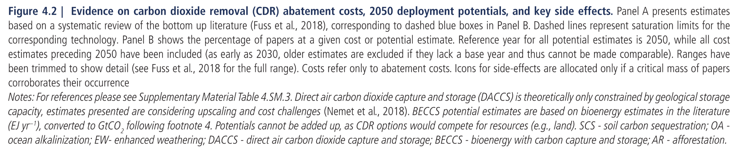
Evidence on carbon dioxide removal (CDR) abatement costs, 2050 deployment potentials, and key side effects
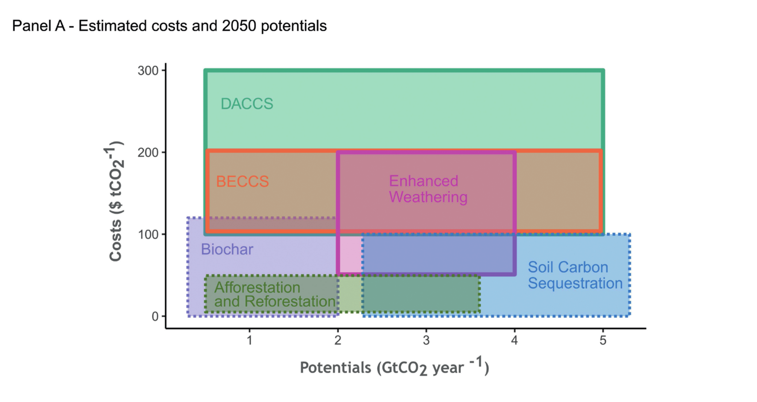
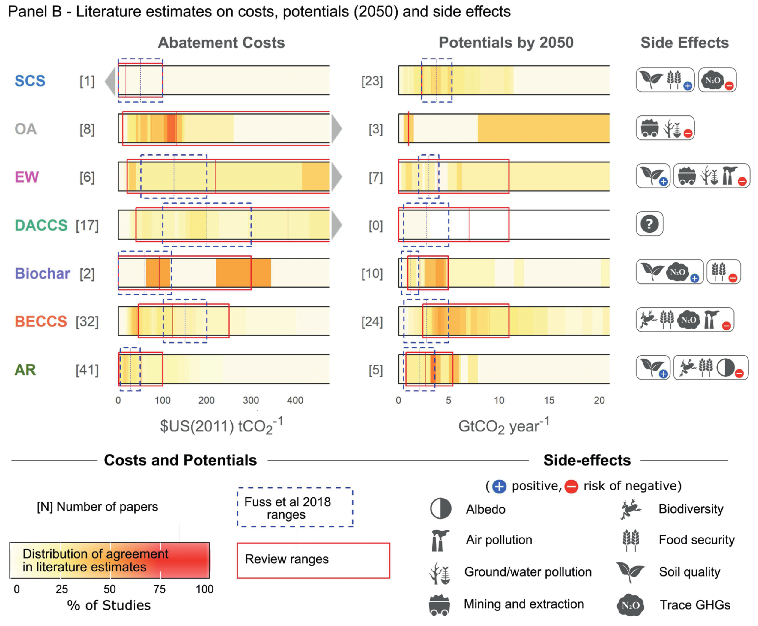
A two-part infographic detailing evidence on carbon dioxide removal abatement costs, 2050 deployment potentials, and key side effects. Panel A uses a chart with overlapping coloured rectangles to map estimated costs in dollars per tonne of CO2 on the vertical axis against potentials in Gigatonnes of CO2 per year on the horizontal axis. Afforestation and Reforestation, Soil Carbon Sequestration, and Biochar generally fall into the lowest cost brackets under 100 dollars. Bioenergy with Carbon Capture and Storage, alongside Enhanced Weathering, span mid-range costs up to 200 dollars, whilst Direct Air Carbon Capture and Storage spans the highest costs up to 300 dollars. Panel B breaks down the literature estimates for seven specific methods using horizontal heatmaps to show where scientific studies agree most strongly on abatement costs and potentials by 2050. The rightmost column displays key side effects using icons to denote positive impacts or risks of negative impacts. For example, Soil Carbon Sequestration and Afforestation are shown to have positive impacts on soil quality, whereas methods like Bioenergy with Carbon Capture and Storage indicate risks of negative impacts on biodiversity, food security, and trace greenhouse gases.

Figure 4.2:  Evidence on carbon dioxide removal (CDR) abatement costs, 2050 deployment potentials, and key side effects. Panel A presents estimates based on a systematic review of the bottom up literature (Fuss et al., 2018), corresponding to dashed blue boxes in Panel B. Dashed lines represent saturation limits for the corresponding technology. Panel B shows the percentage of papers at a given cost or potential estimate. Reference year for all potential estimates is 2050, while all cost estimates preceding 2050 have been included (as early as 2030, older estimates are excluded if they lack a base year and thus cannot be made comparable). Ranges have been trimmed to show detail (see Fuss et al., 2018 for the full range). Costs refer only to abatement costs. Icons for side-effects are allocated only if a critical mass of papers corroborates their occurrence.   Notes: For references please see Supplementary Material Table 4.SM.3. Direct air carbon dioxide capture and storage (DACCS) is theoretically only constrained by geological storage capacity, estimates presented are considering upscaling and cost challenges (Nemet et al., 2018). BECCS potential estimates are based on bioenergy estimates in the literature (EJ yr−1), converted to GtCO2 following footnote 4. Potentials cannot be added up, as CDR options would compete for resources (e.g., land). SCS - soil carbon sequestration; OA - ocean alkalinization; EW- enhanced weathering; DACCS - direct air carbon dioxide capture and storage; BECCS - bioenergy with carbon capture and storage; AR – afforestation.
Source: IPCC (2018) SR15 Chapter 4, Figure 4.2, pg. 344

Summary of status, costs, potentials, risk and impacts, co-benefits, trade-offs and spillover effects and the role in mitigation pathways for CDR methods
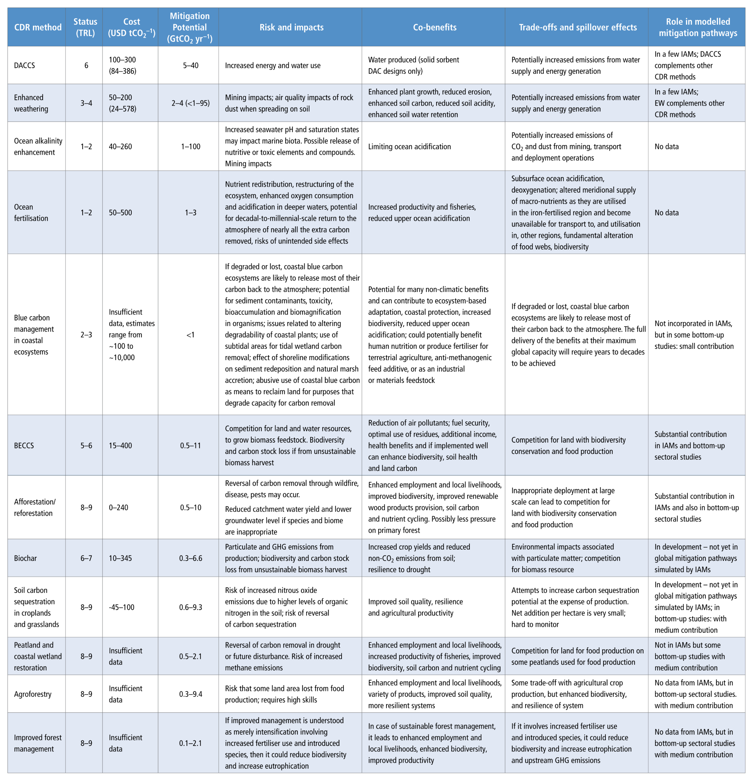

A detailed summary table comparing twelve Carbon Dioxide Removal methods across seven evaluation metrics. The columns detail Status using a Technology Readiness Level score, Cost in US dollars per tonne of CO2, Mitigation Potential in Gigatonnes of CO2 per year, Risks and impacts, Co-benefits, Trade-offs and spillover effects, and Role in modelled mitigation pathways. The methods evaluated span from low-readiness oceanic approaches to high-readiness land management. Low readiness methods scoring 1 to 2 include Ocean alkalinity enhancement and Ocean fertilisation, which face significant risks regarding marine ecosystem impacts. Mid-readiness methods include Direct Air Carbon Capture and Storage, Bioenergy with Carbon Capture and Storage, and Biochar. Direct Air Carbon Capture and Storage shows high costs of 100 to 300 dollars but offers massive mitigation potential of 5 to 40 Gigatonnes. High readiness methods scoring 8 to 9 include Afforestation and reforestation, Soil carbon sequestration, Peatland restoration, Agroforestry, and Improved forest management. These land-based methods generally show lower costs and strong co-benefits like improved biodiversity and local livelihoods, though they share common risks such as carbon reversal through wildfires or land competition with food production.
Table 12.6:  Summary of status, costs, potentials, risk and impacts, co-benefits, trade-offs and spillover effects and the role in mitigation pathways for CDR methods. Technology readiness level (TRL) is a measure of maturity of the CDR method. Scores range from 1 (basic principles defined) to 9 (proven in operational environment). Author judgement ranges (assessed by authors in the literature) are shown, with full literature ranges shown in brackets.
Source: IPCC (2022) AR6 WGIII Chapter 12, Table 12.6, pg. 1275

Characteristics of carbon dioxide removal (CDR) methods, ordered according to the time scale of carbon storage
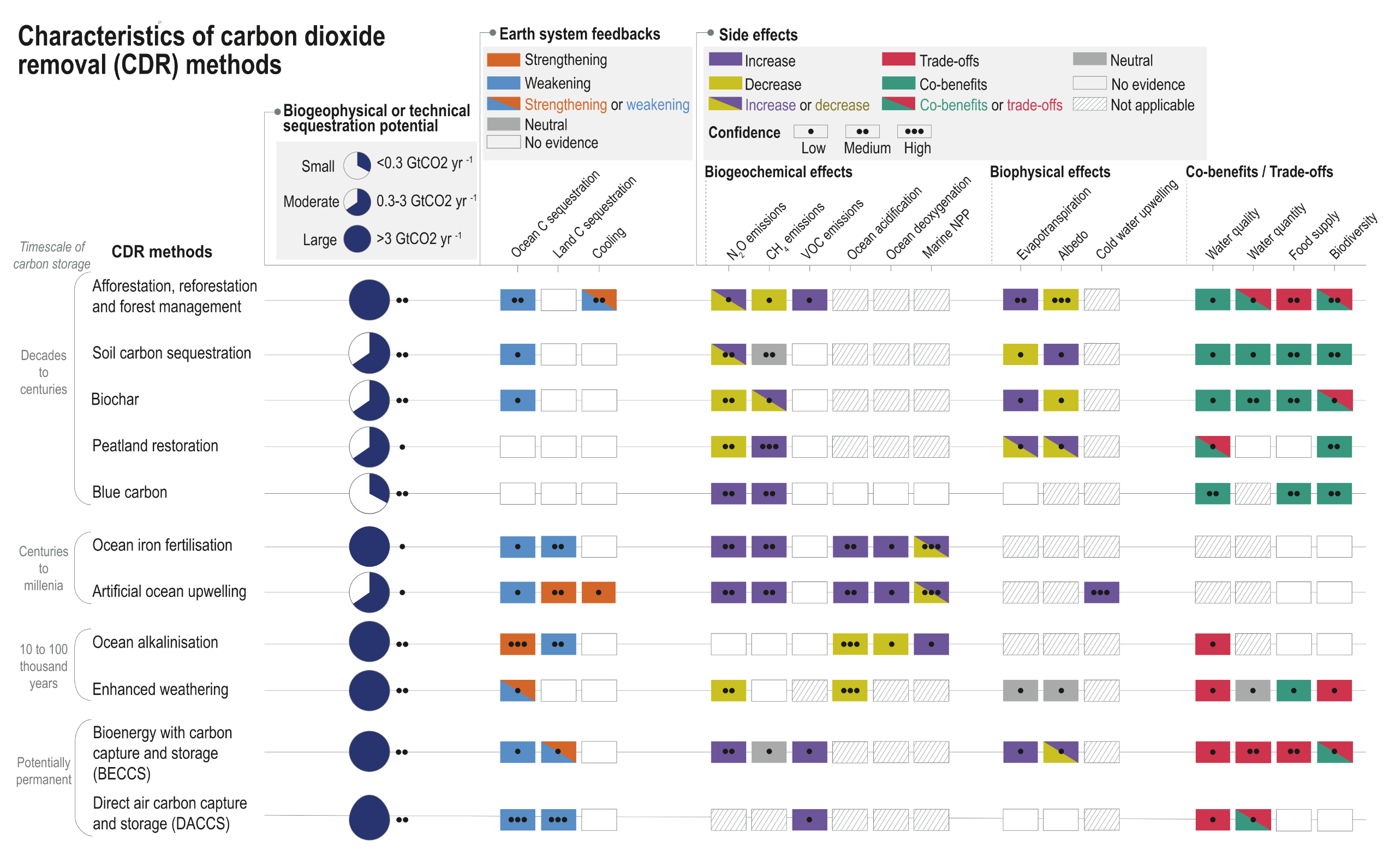

A comprehensive visual table, detailing the characteristics of eleven carbon dioxide removal methods, ordered by their timescale of carbon storage. The table evaluates each method across several columns including sequestration potential, Earth system feedbacks, biogeochemical and biophysical side effects, and co-benefits or trade-offs. Confidence levels for each metric are indicated by one to three dots. Methods are grouped into four timescale categories. Decades to centuries includes afforestation, soil carbon sequestration, biochar, peatland restoration, and blue carbon. These generally offer moderate to large sequestration potentials with many co-benefits, though afforestation poses trade-offs for water quantity and food supply. Centuries to millennia includes ocean iron fertilisation and artificial ocean upwelling, both showing large potentials but driving increased ocean acidification and deoxygenation. Ten to one hundred thousand years includes ocean alkalinisation and enhanced weathering; both have large potentials and show strengthening Earth system feedbacks, but pose trade-offs for water quality. Finally, potentially permanent methods include bioenergy with carbon capture and storage, and direct air carbon capture and storage. Both offer large potentials, but bioenergy with carbon capture presents widespread trade-offs across water, food, and biodiversity, whereas direct air carbon capture shows mostly neutral or not applicable side effects.
Figure 5.36:  Characteristics of carbon dioxide removal (CDR) methods, ordered according to the time scale of carbon storage. The first column shows biogeophysical (for open-ocean methods) or technical (for all other methods) sequestration potentials (i.e., the sequestration potentials constrained by biological, geophysical, geochemical limits and thermodynamics and, for technical potentials, availability of technologies and practices; technical potentials for some methods also consider social or environmental factors if these represent strong barriers for deployment; see Glossary, Annex VII), classified into low (<0.3 GtCO2 yr –1), moderate (0.3−3 GtCO2 yr –1) and large (>3 GtCO2 yr –1) (details underlying this classification are provided in Supplementary Materials Table 5.SM.5). The other columns show Earth system feedbacks that deployment of a given CDR method would have on carbon sequestration and climate, along with biogeochemical, biophysical, and other side effects of a given method. Earth system feedbacks do not include the direct effect of CO2 sequestration on atmospheric CO2, only secondary effects. For Earth system feedbacks, the colours indicate whether the feedbacks strengthen or weaken carbon sequestration and the climate cooling effect of a given CDR method. For biogeochemical and biophysical side effects the colours indicate whether the deployment of a CDR method increases or decreases the magnitude of the effect, whereas for co-benefits and trade-offs the colour indicates whether deployment of a CDR method results in beneficial (co-benefits) or adverse side effects (trade-offs) for water quality and quantity, food production and biodiversity. The details and references underlying the Earth system feedback and side effect assessment are provided in Supplementary Materials Table 5.SM.4. Further details on data sources and processing are available in the chapter data table (Table 5.SM.6).
Source: IPCC (2021) AR6 WGI Chapter 5, Figure 5.36

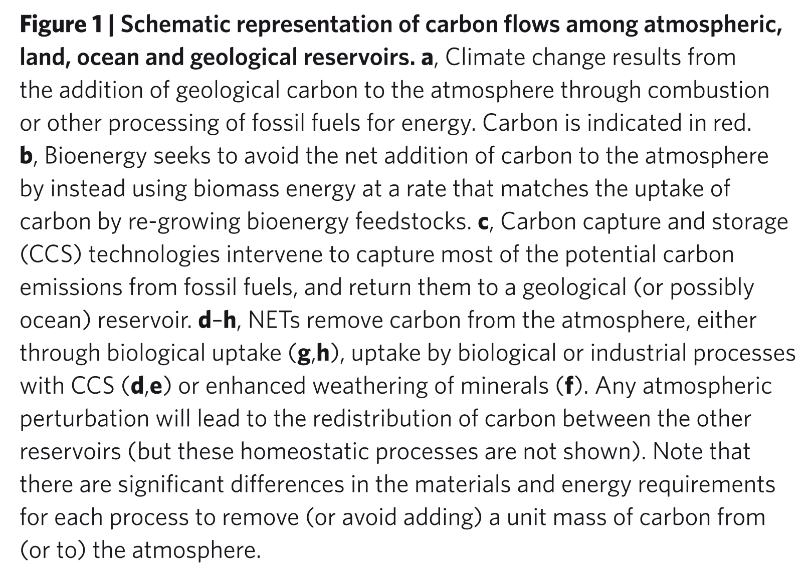
Carbon flows among atmospheric, land, ocean and geological reservoirs
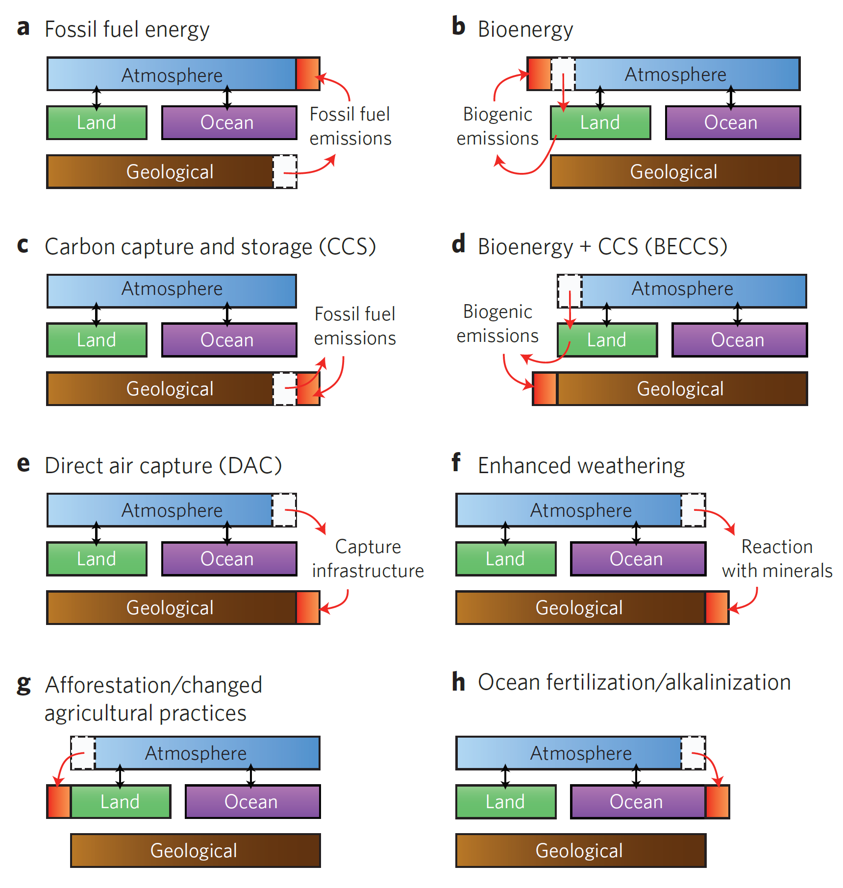
A diagram that uses eight schematic panels, labelled a through h, to illustrate carbon flows among four reservoirs: Atmosphere in blue, Land in green, Ocean in purple, and Geological in brown. Black double-headed arrows show natural homeostasis between the atmosphere, land, and ocean. Red blocks and arrows indicate human-driven carbon movement. Panel a, Fossil fuel energy, shows a flow from the geological reservoir adding a red carbon block to the atmosphere. Panel b, Bioenergy, shows a cyclical biogenic flow between the land and atmosphere. Panel c, Carbon capture and storage, shows fossil fuel emissions from the geological reservoir being captured and returned directly to the geological reservoir. Panels d through h show negative emissions technologies removing carbon from the atmosphere. Panel d, Bioenergy plus carbon capture and storage, moves carbon from the atmosphere to the land via biogenic emissions, and then permanently into the geological reservoir. Panel e, Direct air capture, moves carbon directly from the atmosphere to the geological reservoir using capture infrastructure. Panel f, Enhanced weathering, moves carbon from the atmosphere to the geological reservoir through reactions with minerals. Panel g, Afforestation and changed agricultural practices, moves carbon from the atmosphere into the land reservoir. Panel h, Ocean fertilisation and alkalinisation, moves carbon from the atmosphere into the ocean reservoir.
Figure 1:  Schematic representation of carbon flows among atmospheric, land, ocean and geological reservoirs. a, Climate change results from the addition of geological carbon to the atmosphere through combustion or other processing of fossil fuels for energy. Carbon is indicated in red. b, Bioenergy seeks to avoid the net addition of carbon to the atmosphere by instead using biomass energy at a rate that matches the uptake of carbon by re-growing bioenergy feedstocks. c, Carbon capture and storage (CCS) technologies intervene to capture most of the potential carbon emissions from fossil fuels, and return them to a geological (or possibly ocean) reservoir. d–h, NETs remove carbon from the atmosphere, either through biological uptake (g,h), uptake by biological or industrial processes with CCS (d,e) or enhanced weathering of minerals (f). Any atmospheric perturbation will lead to the redistribution of carbon between the other reservoirs (but these homeostatic processes are not shown). Note that there are significant differences in the materials and energy requirements for each process to remove (or avoid adding) a unit mass of carbon from (or to) the atmosphere.
Source: Smith et al (2016) Biophysical and economic limits to negative CO2 emissions, Figure 1

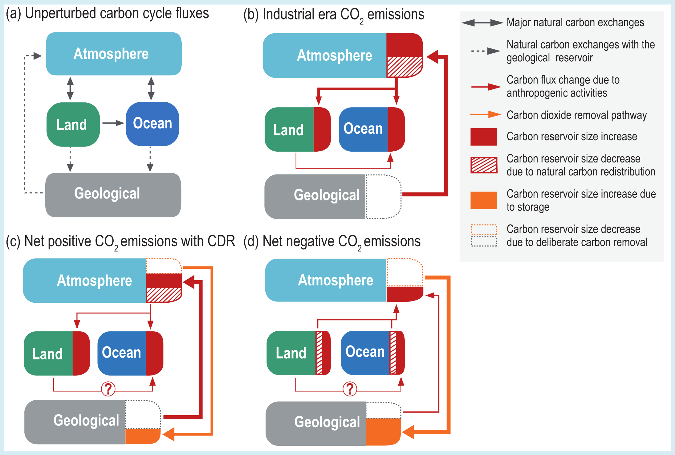
Schematic representation of carbon fluxes between atmosphere, land, ocean and geological reservoirs

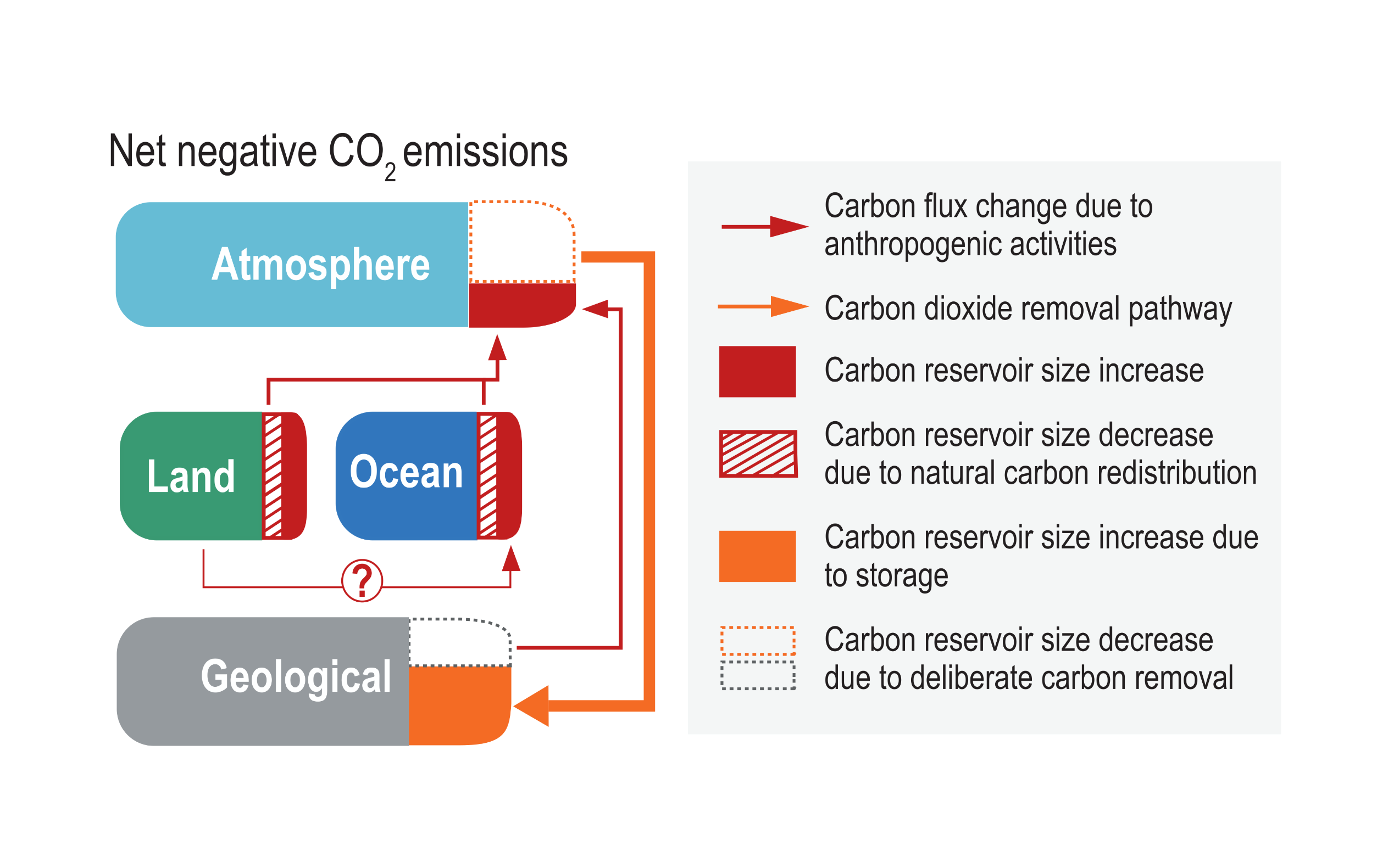
A four-part diagram, illustrating schematic representations of carbon fluxes between atmosphere, land, ocean, and geological reservoirs under different system conditions. The reservoirs are depicted as boxes: Atmosphere in light blue, Land in green, Ocean in dark blue, and Geological in grey. Panel A shows Unperturbed carbon cycle fluxes, with black arrows indicating major natural carbon exchanges between the atmosphere, land, and ocean, and dashed arrows showing natural exchanges with the geological reservoir. Panel B shows Industrial era CO2 emissions. A thick red arrow indicates carbon flux from the geological reservoir to the atmosphere due to anthropogenic activities. Red shaded blocks added to the atmosphere, land, and ocean boxes indicate a carbon reservoir size increase, whilst a dashed outline in the geological box shows a decrease. Panel C shows Net positive CO2 emissions with Carbon Dioxide Removal. It includes the anthropogenic emissions from Panel B, but adds an orange arrow representing a Carbon Dioxide Removal pathway moving carbon from the atmosphere to an orange storage block in the geological reservoir. A question mark sits on the flux line between land and ocean indicating an unknown effect. Panel D shows Net negative CO2 emissions, where the orange Carbon Dioxide Removal pathway from the atmosphere to the geological storage exceeds fossil fuel emissions. Here, hatched regions and dashed outlines in the atmosphere, land, and ocean indicate a carbon reservoir size decrease due to deliberate carbon removal and natural carbon redistribution.
Box 5.3, Figure 1:  Schematic representation of carbon fluxes between atmosphere, land, ocean and geological reservoirs. Different system conditions are shown: (a) an unperturbed Earth system; and changes in carbon fluxes for (b) an Earth system perturbed by fossil fuel carbon dioxide (CO2) emissions; (c) an Earth system in which fossil fuel CO2 emissions are partially offset by carbon dioxide removal (CDR); (d) an Earth system in which CDR exceeds CO2 emissions from fossil fuels (‘net negative’ CO2 emissions). Carbon fluxes depicted in (a) (solid and dashed black lines) also occur in (b–d). The question mark in the land-to-ocean carbon flux perturbation in (c) and (d) indicates that the effect of CDR on this flux is unknown. Note that box sizes do not scale with the size of carbon reservoirs. Adapted from Keller et al. (2018a). Further details on data sources and processing are available in the chapter data table (Table 5.SM.6).
Source: IPCC (2021) AR6 WGI Chapter 5, Box 5.3, Figure 1

Overreliance on BECCS


Many proposals for reaching net-zero emissions this century rely heavily on bioenergy with carbon capture and storage (BECCS). This 2016 Carbon Brief article explains how BECCS became climate change’s ‘saviour’ technology.


IPCC scenarios reliant on BECCS (in 2018)

“Of the 114 scenarios assessed by the IPCC leading to forcing values of around 2.6 Wm−2 (likely probability for 2°C), 104 show net CDR in the second half of the century, mostly achieved by bioenergy with CCS (BECCS)”

Source: van Vuuren et al (2018)


A decarbonisation scenario that avoids BECCS.

“This analysis shows that alternative pathways exist allowing for more moderate use and postponement of BECCS”. Bioenergy with carbon capture and storage (BECCS) can “be limited by a range of societal and technological factors and choices” … “A rapid transformation in energy consumption and land use is needed in all scenarios”

Source: van Vuuren et al (2018)


Scenarios and assumptions
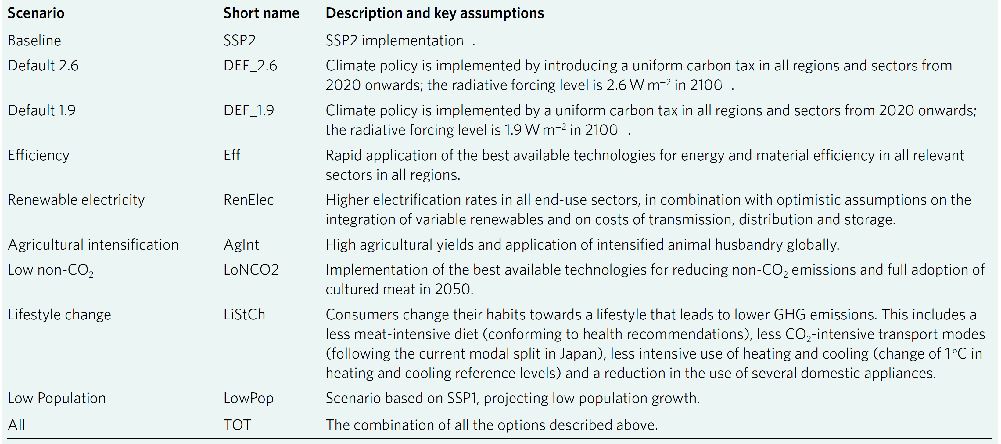
A detailed data table, outlining ten different climate scenarios and their underlying assumptions. The table features three columns: Scenario, Short name, and Description and key assumptions. The Baseline scenario, short name SSP2, assumes standard SSP2 implementation. Default 2.6, short name DEF_2.6, assumes a uniform carbon tax from 2020 onwards, targeting a radiative forcing level of 2.6 Watts per square metre by 2100. Default 1.9, short name DEF_1.9, is identical but targets a stricter 1.9 Watts per square metre. The Efficiency scenario, short name Eff, focuses on the rapid global application of the best available technologies for energy and material efficiency. Renewable electricity, short name RenElec, assumes higher electrification rates alongside optimistic assumptions regarding variable renewables, transmission, and storage costs. Agricultural intensification, short name AgInt, assumes high agricultural yields and intensified animal husbandry globally. Low non-CO2, short name LoNCO2, assumes the best available technologies for reducing non-CO2 emissions and the full global adoption of cultured meat by 2050. Lifestyle change, short name LiStCh, assumes consumers adopt lower greenhouse gas habits, such as less meat-intensive diets, less CO2-intensive transport modes, a 1 degree Celsius reduction in heating and cooling reference levels, and reduced domestic appliance use. Low Population, short name LowPop, projects low population growth based on the SSP1 pathway. Finally, the All scenario, short name TOT, represents the simultaneous combination of all the previously described mitigation options, which the study notes is the only pathway that theoretically avoids the need for Bioenergy with Carbon Capture and Storage.
Source: van Vuuren et al (2018), Table 1

Avoiding reliance on BECCS by decarbonising via alternative pathways

A stacked bar chart, displaying global primary energy use in Exajoules per year for the years 2010, 2050, and 2100 across nine different climate mitigation scenarios. The vertical axis ranges from 0 to 1000 Exajoules per year. The bars are colour-coded by energy source, including coal, oil, gas, nuclear, hydro, solar and wind, traditional biomass, modern biomass, and modern bioenergy with carbon capture and storage, alongside fossil fuels paired with carbon capture and storage. The single 2010 baseline bar shows approximately 500 Exajoules per year, heavily dominated by unabated coal, oil, and gas. By 2050 and 2100, the scenarios illustrate a massive transition towards renewables and bioenergy. In most pathways, such as the default 1.9 and 2.6 scenarios, modern bioenergy with carbon capture and storage, visualised in dark green at the base of the bars, makes up a significant and growing portion of the primary energy mix. Crucially, the Total scenario, which models the combination of all alternative mitigation options, demonstrates a pathway with the lowest overall energy demand. By 2100, the energy mix in the Total scenario relies almost entirely on solar and wind power, shown in yellow, and modern biomass, shown in bright green, successfully achieving deep decarbonisation with zero reliance on modern bioenergy with carbon capture and storage.
Source: van Vuuren et al (2018) Alternative pathways to the 1.5°C target reduce the need for negative emission technologies, Fig. 3C

Trad.Bio: traditional bioenergy
Mod.Bio: modern bioenergy
Mod.BECCS: modern BECCS

The baseline for this scenario is IPCC’s ‘SSP2’ ‘Middle of the road’.

The primary energy mix is mostly solar and wind in 2100, with a continued reliance on gas, gas with CCS, coal with CCS, oil, and nuclear power.

Key point: there’s no BECCS in the ‘Total’ scenario (which combines the other scenarios in this study).


World can limit global warming to 1.5C ‘without BECCS’


Analysis: How ‘natural climate solutions’ can reduce the need for BECCS


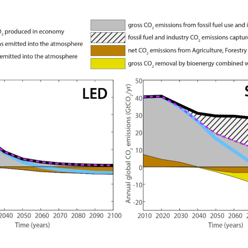
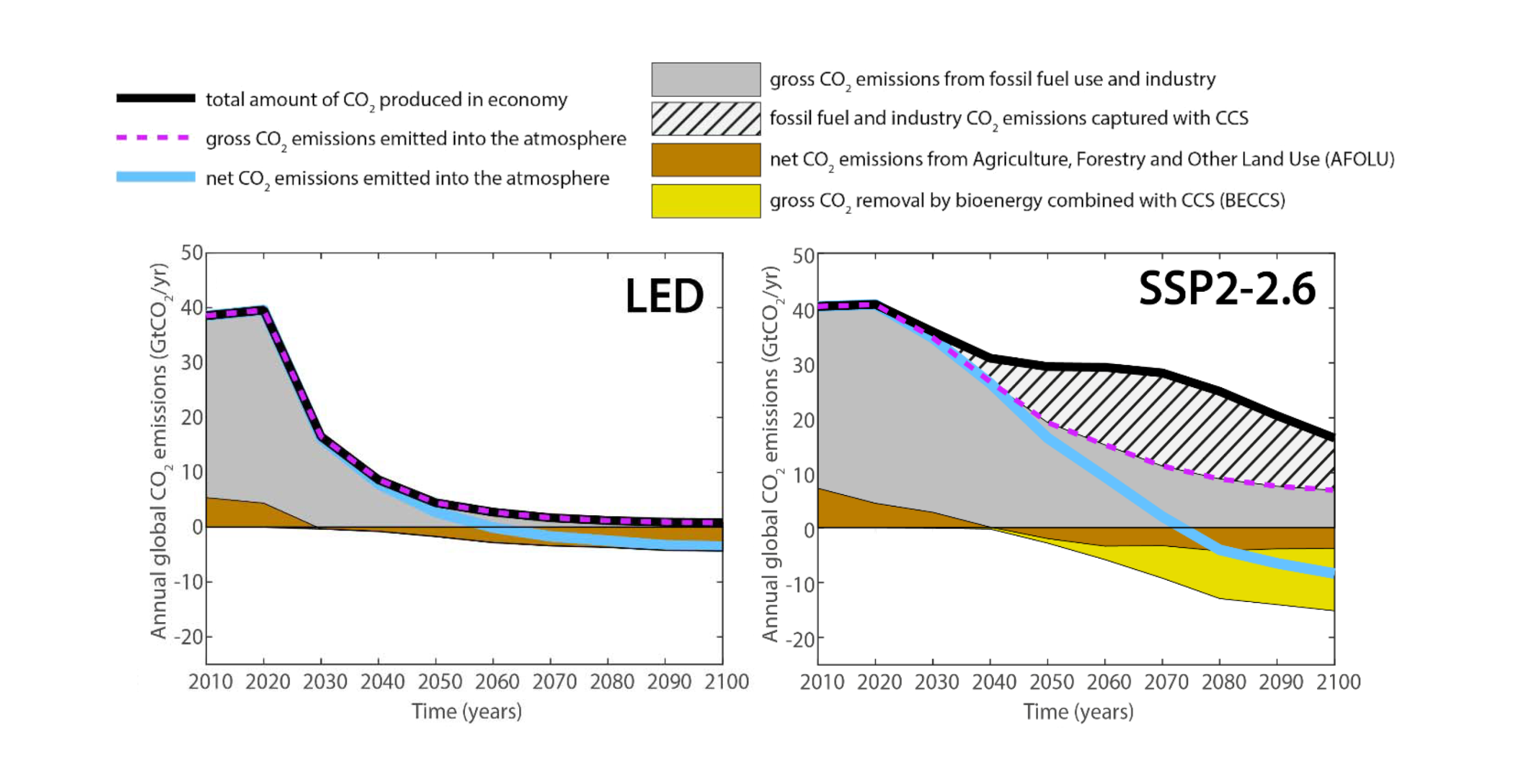
Low Energy Demand Scenario needs no BECCS and needs less decarbonisation effort
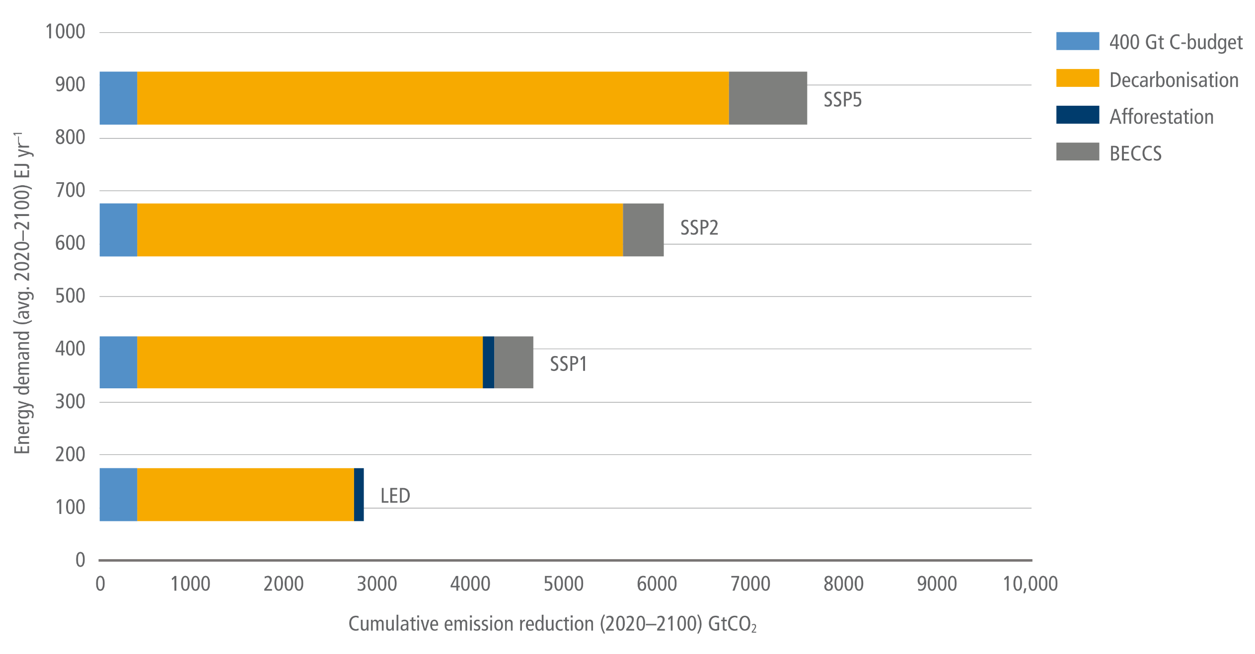
A horizontal stacked bar chart, illustrating how the required climate mitigation effort scales with global energy demand. The vertical axis represents average global final energy demand from 2020 to 2100 in Exajoules per year, ranging from 0 to 1000. The horizontal axis measures cumulative emission reduction from 2020 to 2100 in Gigatonnes of CO2, ranging from 0 to 10000. Four scenarios are plotted: LED, SSP1, SSP2, and SSP5, positioned at increasing levels of energy demand. Each bar is divided into colour-coded mitigation components: a baseline 400 Gigatonne carbon budget in light blue, Decarbonisation in yellow, Afforestation in dark blue, and BECCS in grey. The chart clearly shows that as energy demand increases from the LED scenario up to SSP5, the total required cumulative emission reduction expands massively from under 3000 to over 7000 Gigatonnes. Consequently, the yellow Decarbonisation segment grows substantially in higher demand scenarios. Crucially, the LED or Low Energy Demand scenario at the bottom relies only on the carbon budget, decarbonisation, and a small sliver of afforestation, completely avoiding any use of BECCS. Conversely, the higher energy scenarios, SSP1, SSP2, and SSP5, require increasingly large grey segments of BECCS to meet the climate target.
Figure 5.1:  Low Energy Demand Scenario needs no BECCS and needs less decarbonisation effort. Dependence of the size of the mitigation effort to reach a 1.5°C climate target (cumulative GtCO2 emission reduction 2020–2100 by option) as a function of the level of energy demand (average global final energy demand 2020–2100 in EJ yr –1) in baseline and corresponding 1.5°C scenarios (1.9 W m–2 radiative forcing change) based on the IPCC Special Report on Global Warming of 1.5°C (data obtained from the Scenario Explorer database, LED baseline emission data obtained from authors). In this figure an example of remaining carbon budget of 400 Gt has been taken from Rogelj et al. (2019) for illustrative purposes. 400 Gt is also the number given in Table SPM.2 (IPCC 2021, p. 29) for a probability of 67% to limit global warming to 1.5°C.
Source: IPCC (2022) AR6 WGIII Chapter 5, Figure 5.1

Solar radiation modification (SRM)


“SRM contrasts with climate change mitigation activities, such as emissions reductions and CDR, as it introduces a ‘mask’ to the climate change problem by altering Earth’s radiation budget, rather than attempting to address the root cause of the problem, which is the increase in GHGs in the atmosphere. By masking only the climate effects of GHG emissions, SRM does not address other issues related to atmospheric CO2 increase, such as ocean acidification.”

Source: IPCC (2021) AR6 WGI, Technical Summary, Box TS.8


“the most commonly studied approaches attempt to mimic the cooling effects of major volcanic eruptions by injecting reflective aerosols (e.g., sulphate aerosols) or their precursors (e.g., sulphur dioxide) into the stratosphere.”

Source: IPCC (2021) AR6 WGI, Technical Summary, Box TS.8


Solar radiation modification (SRM) “Refers to a range of radiation modification measures not related to greenhouse gas (GHG) mitigation that seek to limit global warming. Most methods involve reducing the amount of incoming solar radiation reaching the surface, but others also act on the longwave radiation budget by reducing optical thickness and cloud lifetime.”

Cirrus cloud thinning (CCT)
“One of several radiation modification approaches to counter the warming caused by greenhouse gases (GHGs). In this approach, it is proposed to reduce the amount of cirrus clouds by injecting ice nucleating substances in the upper troposphere. The reduction in cirrus clouds is expected to increase the amount of longwave cooling to space resulting in a planetary cooling. Although cirrus cloud thinning primarily affects the longwave radiation budget of our planet, it is often identified as one of the solar radiation modification (SRM) approaches in the literature.”

Marine cloud brightening (MCB)
“One of several solar radiation modification (SRM) approaches to increase the planetary albedo. In this approach, it is proposed to inject sea salt aerosols into persistent marine low clouds. This is expected to increase the cloud droplet concentration of these clouds and their reflectivity.”

Stratospheric aerosol injection (SAI)
“One of several solar radiation modification (SRM) approaches to increase the planetary albedo. In the approach, it is proposed to inject highly reflective aerosols such as sulphates into the lower stratosphere. This is expected to increase the fraction of solar radiation deflected to space resulting in a planetary cooling.”

Source: IPCC (2021) AR6 WGI Annex VII, Glossary, pg. 2249


A summary of the various SRM approaches
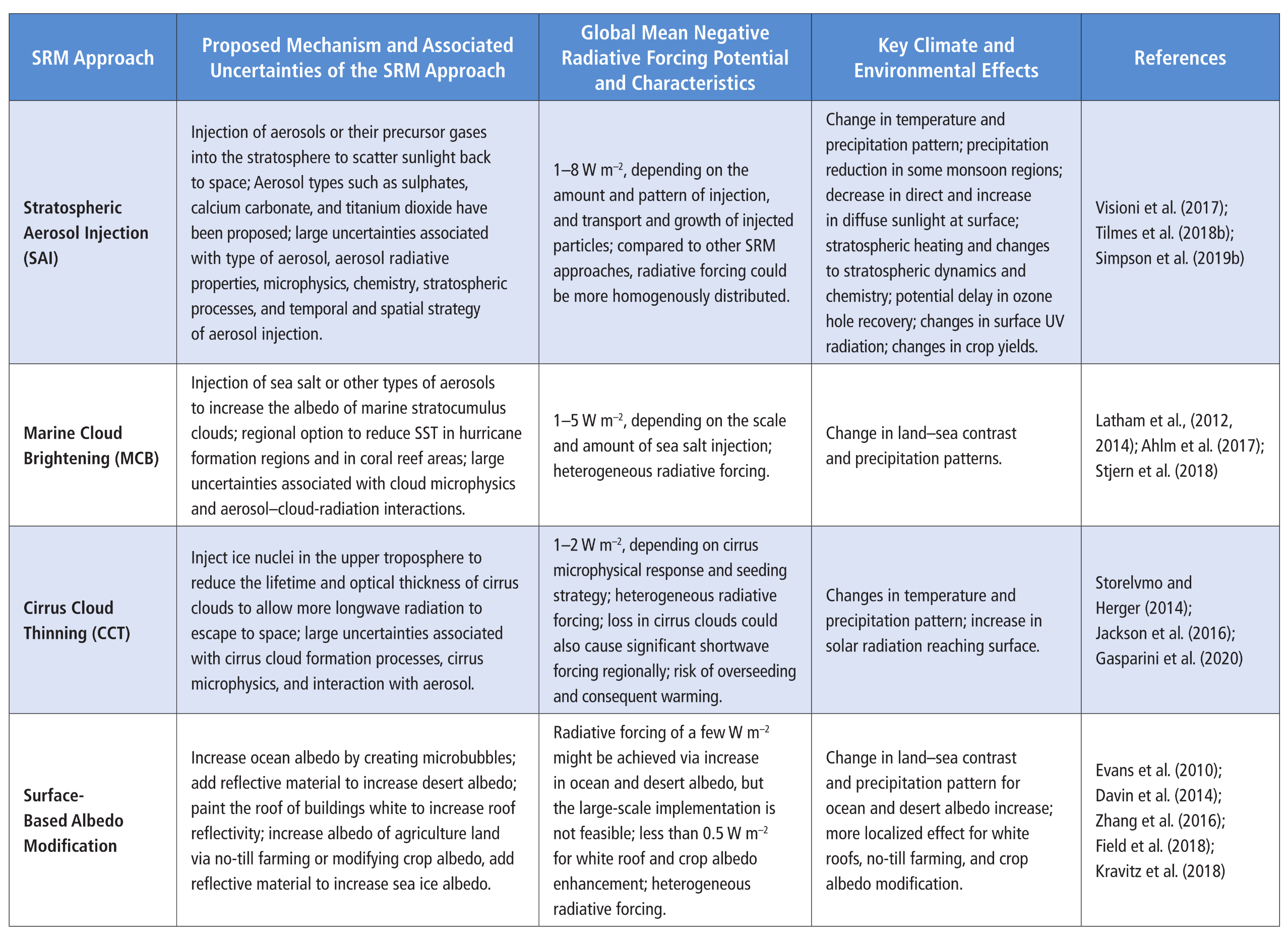
A detailed summary table, outlining four Solar Radiation Modification approaches. The table features five columns: SRM Approach, Proposed Mechanism and Associated Uncertainties, Global Mean Negative Radiative Forcing Potential and Characteristics, Key Climate and Environmental Effects, and References. The first approach, Stratospheric Aerosol Injection, involves injecting aerosols like sulphates into the stratosphere to scatter sunlight back to space. This could provide 1 to 8 Watts per square metre of negative forcing, but risks stratospheric heating, delayed ozone hole recovery, and changes in crop yields. The second, Marine Cloud Brightening, involves injecting sea salt to increase the albedo of marine stratocumulus clouds, yielding 1 to 5 Watts per square metre of heterogeneous forcing, which may alter land-sea contrast and precipitation patterns. The third, Cirrus Cloud Thinning, injects ice nuclei in the upper troposphere to reduce cirrus cloud thickness, allowing more longwave radiation to escape. This offers 1 to 2 Watts per square metre of forcing but carries a risk of overseeding and consequent warming. The final approach, Surface-Based Albedo Modification, includes increasing the reflectivity of oceans, deserts, roofs, agriculture land, and sea ice. Ocean and desert modifications might achieve a few Watts per square metre, whilst white roofs and crop modifications offer less than 0.5 Watts per square metre, producing more localised climate and environmental effects.
Source: IPCC (2021) AR6 WGI, Chapter 4, Table 4.7, pg. 624

“SRM could offset some of the effects of increasing greenhouse gases on global and regional climate, including the carbon and water cycles (high confidence). However, there would be substantial residual or overcompensating climate change at the regional scales and seasonal time scales (high confidence), and large uncertainties associated with aerosol–cloud–radiation interactions persist. The cooling caused by SRM would increase the global land and ocean CO2 sinks (medium confidence), but this would not stop CO2 from increasing in the atmosphere or affect the resulting ocean acidification under continued anthropogenic emissions (high confidence).”

Source: IPCC (2021) AR6 WGI, Technical Summary, Box TS.8


“It is likely that abrupt water cycle changes will occur if SRM techniques are implemented rapidly. A sudden and sustained termination of SRM in a high CO2 emissions scenario would cause rapid climate change (high confidence). However, a gradual phase-out of SRM combined with emissions reduction and carbon dioxide removal (CDR) would avoid these termination effects (medium confidence).”

Source: IPCC (2021) AR6 WGI, Technical Summary, Box TS.8


“There is high agreement in the literature that for addressing climate change risks SRM is, at best, a supplement to achieving sustained net zero or net negative CO2 emission levels globally.”

Source: IPCC (2022) AR6 WGII, Technical Summary, Section TS.C.13.4, pg. 69


Sources for this post:


Featured image: IPCC (2021) AR6 WGI Chapter 5, Box 5.3, Figure 1 (modified)